Transformer architecture.

Attention is all you need

Attention is All You Need is a seminal paper in the field of natural language processing (NLP) and deep learning, introducing the Transformer architecture. Published by Vaswani et al. in 2017, it revolutionized sequence-to-sequence tasks by replacing recurrent and convolutional layers with self-attention mechanisms.The overall architecture of Transformer architecture is discussed below:

Tokenization

Tokenization is like taking a sentence and breaking it down into smaller parts, like words or even parts of words.

Why tokenize?

Computers understand small parts better: It’s easier for a computer to understand individual words or parts of words than a whole sentence at once.
We can analyze language: By looking at the tokens, we can understand how words are used and what they mean.
It helps with tasks: Things like machine translation, writing different kinds of creative text formats, and answering your questions all use tokenization!

How to tokenize?

There are different ways to break down a sentence:

By word: This is the easiest way. We just separate the words based on spaces, like in our Lego example.
By parts of words: Sometimes, we break words into smaller parts, like “unbreakable” into “un,” “break,” and “able.” This helps with unusual words.
By character: We can even break down words into individual letters! This is useful for languages with complex writing systems.

Example:

Input Sentence: Nepal is a beautiful country

Tokenization Method: Word-based (splitting on spaces and punctuation) - for now, let’s not used punctuation like fullstop.

Tokens:

Nepal
is
a
beautiful
country

Note: This is a basic example of word-based tokenization for easy understanding. Other methods, like Byte Pair Encoding(BPE) or character-based tokenization, would produce different token sequences. For more details on tokenization, please visit Tokenization Lecture by Andrej Karpathy

Input ID

In natural language processing (NLP), a vocabulary, also known as a dictionary or lexicon, is a finite set of all unique words or tokens that can appear in a given corpus or dataset.
It essentially represents the entire set of words that the NLP model is trained on or expected to encounter during its tasks.
Once the text has been tokenized, a vocabulary is created by compiling a list of unique tokens present in the dataset. Each token is assigned a unique index or identifier within the vocabulary.
For example, the vocabulary might look like {“Nepal”: 4858, “is”: 785, “a”: 2, “beautiful”: 563, “Country”: 975}. This mapping allows the model to represent words as numerical indices, which can then be efficiently processed during training and inference.

Input Embeddings

It involves representing words or tokens from a vocabulary as dense, continuous-valued vectors. These vectors capture semantic information about the tokens, enabling the model to understand and process the input data effectively.
The integer indices are passed through an embedding layer. This layer is initialized with random values and learns to map each index to a continuous vector during training. Each index corresponds to a row in the embedding matrix, and the layer retrieves the corresponding vector for each input token.
The dimension of the input embedding vectors is 512 in the original transformer paper. This means that each token in the input sequence is represented by a dense vector of length 512 after passing through the embedding layer.

Positional Encodings

RNNs leverage recurrent connections and hidden states to capture temporal dependencies and process sequential data dynamically, while CNNs use convolutional filters to capture local patterns and hierarchical features in sequential data, treating the sequence as a one-dimensional signal.In case of transformers the input is provided all at once and not word by word. Hence, the position of each word needs to be explicitly provided and is called as positional encoding. But how do we provide the positions of each words/tokens to the transformer? some of the criterias that must be satisfied by positional encodings are :

1. Unique Encoding for Each Time-step:

This criterion ensures that each position in the sequence has a distinct encoding. This is important because different positions in the sequence may convey different contextual information. For example, in a sentence, the word “cat” appearing at the beginning should have a different encoding than the same word appearing later in the sentence.

2. Consistent Distance Between Time-steps Across Sentences:

This ensures that the positional encodings maintain consistent relationships between different positions across sequences of varying lengths. It means that the distance between any two time-steps should represent the same relative distance in the sequence, regardless of the sequence length. For example, if the distance between time-step 1 and time-step 2 is 0.5 for a sequence of length 4, then for a sequence of length 8, the distance between time-step 1 and time-step 2 should also be 0.5.

3. Generalization to Longer Sentences Without Effort:

This criterion implies that the positional encodings should be scalable and adaptable to sequences of different lengths without requiring additional adjustments or training efforts. For example, if a model trained on sentences of length up to 10 can generalize well to sentences of length 20 without retraining, it indicates that the positional encodings are effective in handling longer sequences.

4. Bounded Values:

Bounded values ensure that the positional encodings do not grow excessively large or small as the sequence length increases, which can help stabilize the training process. For example, if the positional encodings are bounded within a range [-1, 1], it prevents numerical instability issues during training.

5. Deterministic Nature:

Deterministic positional encodings ensure that for a given position in the sequence, the encoding is always the same, regardless of other factors. This property is essential for reproducibility and consistency in model training and inference. For example, if the positional encoding for the word “cat” at position 3 in a sentence is always the same, regardless of the content of the sentence or the training instance.

To meet these criterias,authors of the original paper proposed a brilliant positional encoding method, such as the sinusoidal positional encoding used in transformer models, employ mathematical functions like sine and cosine to generate deterministic encodings that satisfy the uniqueness, consistency, generalization, boundedness, and deterministic nature required for effective sequence processing.

How is it accomplished?

Imagine we have a sentence with 5 words.

Nepal is a beautiful Country

Each word is represented by a 512-dimensional embedding vector.

We want to add positional encoding to each word embedding to incorporate information about their position in the sentence.

pos: This represents the position of the word in the sentence. It ranges from 0 to 4 in our 5-word sentence example.
i: This represents the dimension of the embedding vector. It ranges from 0 to 511 for a 512-dimensional vector.
d_model: This is the total dimensionality of the word embedding, which is 512 in our example.

Let’s generate the positional encoding vector for the 4th word “beautiful” (position pos = 3 as pos starts from 0) in an input sentence with a 512-dimensional embedding and encoding space (d_model = 512).

Formulas for d_model = 512:

Even dimensions (2i): PE_(3, 2i) = sin(3 / 10000^(2i/512))
Odd dimensions (2i+1): PE_(3, 2i+1) = cos(3 / 10000^(2i/512))

Dimension Index (i)	Formula	Value (approx.)
0	sin(3 / 10000^0)	0.0003
1	cos(3 / 10000^0)	0.999999999
2	sin(3 / 10000^(4/512))	0.0006
3	cos(3 / 10000^(6/512))	0.999999998
---	---	---
---	---	---
---	---	---
255	cos(3 / 10000^(510/512))	-0.7071
256	sin(3 / 10000^(512/512))	0.7071

Resulting Vector (Example):

[0.0003, 0.999999999, 0.0006, 0.999999998, …, -0.7071, 0.7071]

This vector would then be added element-wise to the 4th word’s embedding vector to incorporate positional information.

Encoder

The Encoder block is a crucial component within the Transformer architecture. It’s responsible for processing and refining input sequences, extracting meaningful information and relationships within the data.Imagine you’re reading a sentence. As you read each word, you subconsciously consider its relationship with the surrounding words to understand the meaning of the sentence. The Encoder block works similarly, analyzing the connections between words in the input sequence to extract a comprehensive understanding of the information.In essence, the Encoder block is crucial for understanding the context and meaning of input sequences. It achieves this by:

Analyzing relationships between words: The self-attention mechanism allows the model to learn how each word relates to others in the sequence, providing context and deeper meaning.
Extracting features: The feed-forward network processes this information to extract complex features and patterns.
Preparing information for further processing: The refined output is then ready for subsequent stages in the Transformer model, like the Decoder block in architectures with encoder-decoder structure.

The individual components of the encoder blocks are described below:

Self Attention

Imagine you’re reading a sentence and trying to understand the meaning of each word. You wouldn’t just look at the word itself; you’d also consider its context, the words around it, and how they relate to each other. Self-attention is a mechanism that allows a machine learning model to do something similar.Self-attention helps a model analyze a sequence (like a sentence) and understand the relationships between different elements within that sequence. It allows each element to “attend” to other relevant elements and gather information that helps capture the context and meaning.

How it Works (Simplified):

Input Sequence: The model receives a sequence as input, such as a sentence with individual words.
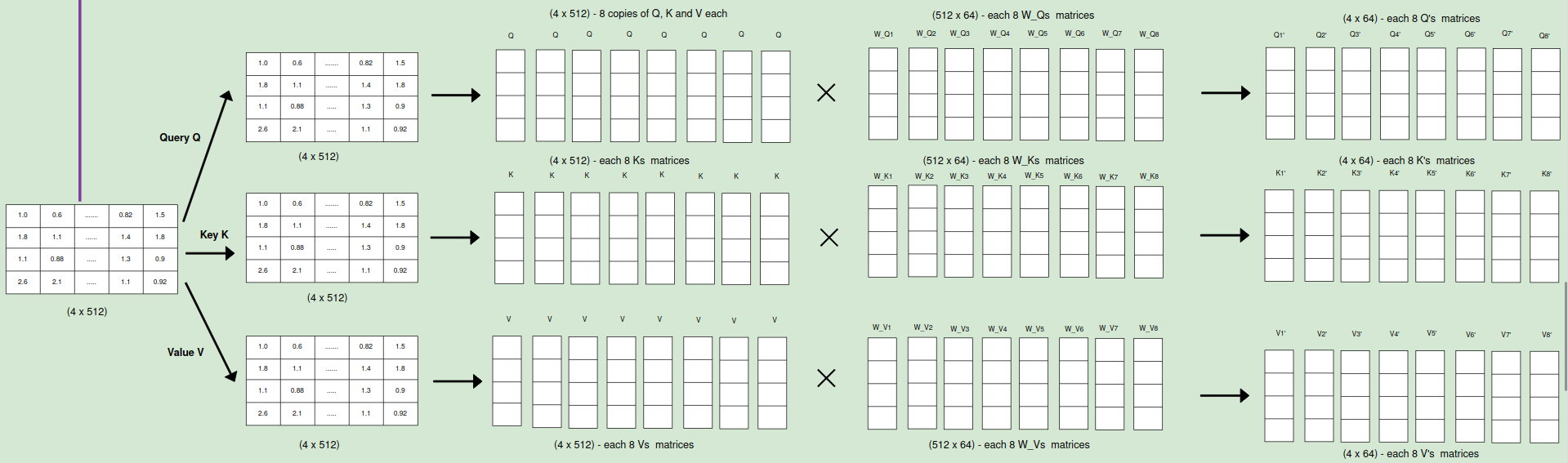
Creating Queries, Keys, and Values: For each word in the sentence, the model creates three vectors:
- Query: Represents what the word is “looking for” or interested in.
- Key: Represents the essential information of another word.
- Value: Represents the actual content of another word.
Attention Scores: The model compares the query of each word with the keys of all other words to calculate attention scores. These scores reflect how relevant each word is to the current word.
Softmax and Weighted Sum: The attention scores are normalized using the softmax function to create a probability distribution. These probabilities are then used as weights to create a weighted sum of the value vectors.
Context Vector: The resulting weighted sum is a context vector that captures relevant information from other words in the sentence, providing a richer representation of the current word’s meaning and context.

Multi Head Attention

1st analogy : Imagine having multiple friends listening to the same conversation, each focusing on different aspects and drawing their own conclusions. That’s the essence of multi-head attention! It enhances the self-attention mechanism by allowing the model to attend to information from different representation subspaces at the same time.Multi-head attention is like having multiple attention mechanisms working in parallel, each with its own set of parameters and focusing on different aspects of the input sequence. This allows the model to capture a richer and more diverse understanding of the relationships between words.

2nd analogy : Think of a group of experts analyzing a piece of art. Each expert focuses on different aspects, such as the brushstrokes, the composition, or the historical context. By combining their insights, they gain a more comprehensive understanding of the artwork. Similarly, multi-head attention allows the model to combine perspectives from different heads to build a richer representation of the input sequence.

The authors found that instead of performing a single attention function with high-dimensional keys, values, and queries, it is more beneficial to project them into multiple lower-dimensional spaces and perform attention in parallel. This allows the model to attend to information from different representation subspaces at different positions, which is inhibited with a single attention head due to averaging.

How it Works?

1. Linear Projections:

The queries (Q), keys (K), and values (V) are each linearly projected h times with different, learned linear projections. This means there are h sets of weight matrices: W_Qi, W_Ki, and W_Vi, each projecting Q, K, and V into a lower-dimensional space of dk, dk, and dv dimensions, respectively. The original paper used h = 8 parallel attention layers or heads.

2. Parallel Attention:

For each of the h projected versions of queries, keys, and values, the attention function is performed in parallel. This means each head independently calculates attention scores, applies softmax to get attention weights, and computes a weighted sum of the values to obtain a dv-dimensional output vector.

3. Concatenation and Final Projection:

The dv-dimensional output vectors from all h heads are concatenated together. A final linear projection, W_O, is applied to the concatenated vector to map it back to the original d_model dimension.

Benefits of Multi-Head Attention:

Diverse Representation: Each head can learn to focus on different types of relationships between words, such as syntactic dependencies, semantic similarities, or long-range connections.
Increased Capacity: By having multiple heads, the model’s capacity to learn complex patterns and relationships within the sequence is increased.By learning different projection matrices for each head, the model can attend to various aspects of the input, leading to a more nuanced understanding of the data.
Improved Robustness: If one head fails to capture certain information, other heads can compensate, leading to a more robust and reliable model.
Computational Efficiency: Attention calculations for different heads can be performed in parallel, leading to faster and more efficient processing. Although multiple attention calculations are performed, the lower dimensionality of each head keeps the overall computational cost similar to that of single-head attention with full dimensionality.

In the original paper, they used dk = dv = d_model/h = 64. This means each head operated on a much smaller dimension (64) compared to the full d_model(512) dimension, making the computations more efficient while still allowing for the benefits of multi-head attention.

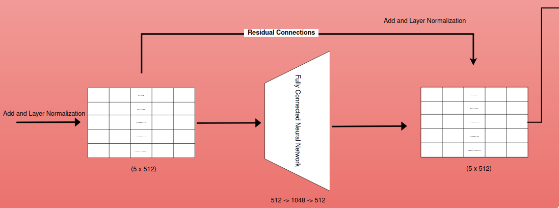
Residual Connection and Layer Normalization

Residual Connection

Concept: Residual connections address the problem of vanishing/exploding gradients, which can occur in deep neural networks during backpropagation. They provide a “shortcut” for the gradient to flow directly through the network, bypassing some layers.
Implementation: A residual connection adds the input of a layer to its output before passing it to the next layer. This can be represented as: y = F(x) + x where:

x is the input to the layer

F(x) is the output of the layer after its transformations

y is the output with the residual connection

What are the benefits of Residual Connections?

Gradient Flow: Residual connections allow gradients to flow more easily during backpropagation, mitigating the vanishing/exploding gradient problem.
Training Deep Networks: This enables the training of deeper networks that would otherwise be difficult due to vanishing gradients.
Improved Performance: Residual connections often lead to improved performance and faster convergence during training.

Layer Normalization

Concept: Layer normalization is a technique for normalizing the activations of a layer, ensuring they have a mean of 0 and a standard deviation of 1. This helps stabilize the distribution of activations and prevent them from becoming too large or too small during training.
Implementation:

Calculate Mean and Variance: For each training example, the mean and variance of the activations within a layer are calculated.
Normalization: The activations are then normalized by subtracting the mean and dividing by the standard deviation.
Scaling and Shifting: Learnable parameters (gain and bias) are introduced to scale and shift the normalized activations, allowing the model to learn the optimal scale and distribution for each layer.

Residual Connection and Layer Normalization

Benefits:

Reduced Internal Covariate Shift: Layer normalization helps reduce the internal covariate shift problem, where the distribution of activations changes during training, leading to instability and slower convergence.
Faster Training: By stabilizing the activations, layer normalization often leads to faster training and improved convergence.
Improved Generalization: It can also lead to better generalization performance, as the model becomes less sensitive to the specific distribution of the training data.

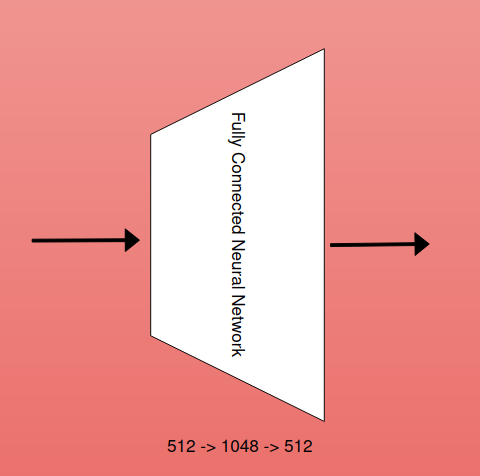
Fully Connected Neural Networks

Following the multi-head attention block in the Transformer architecture, the contextualized representation is passed through a fully connected feedforward network (FFN) to further enhance its expressiveness and capture non-linear relationships within the sequence.The FFN consists of two linear transformations with a ReLU (Rectified Linear Unit) activation function in between.

The first linear layer(hidden layer) projects the input(512d) into a higher-dimensional space. In the original Transformer paper, this hidden layer has a dimensionality of 2048, regardless of the embedding dimension (which is 512).
The second linear layer projects the output of the hidden layer back to the original embedding dimension (512 in this case).

Benefits of the Feedforward Network:

Non-Linearity: The FFN adds non-linearity to the model, enabling it to learn complex patterns and relationships that go beyond simple linear combinations of features.
Increased Expressiveness: The higher-dimensional hidden layer allows the model to capture more nuanced interactions between features and extract richer representations of the input sequence.
Position-wise Transformations: The FFN operates independently on each position in the sequence, allowing for position-specific adjustments and fine-tuning of the representations.

Residual Connection and Layer Normalization

Concepts and explanations - Same as explained before.

Both residual connections and layer normalization are used extensively in Transformer models.They work together to improve training stability and performance, allowing for the training of deep models with numerous layers and complex architectures.

Encoder Blocks

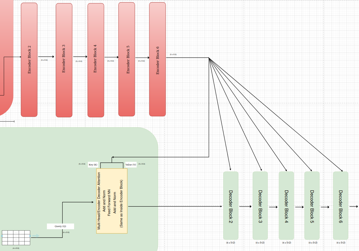
The Transformer encoder is composed of a stack of identical encoder blocks, typically with 6 blocks in the original architecture. Each block processes the input sequence and refines the representation through a series of operations, culminating in a final output that captures rich contextual information.The output of one block becomes the input to the next block, allowing for a hierarchical and progressively deeper representation of the input sequence.

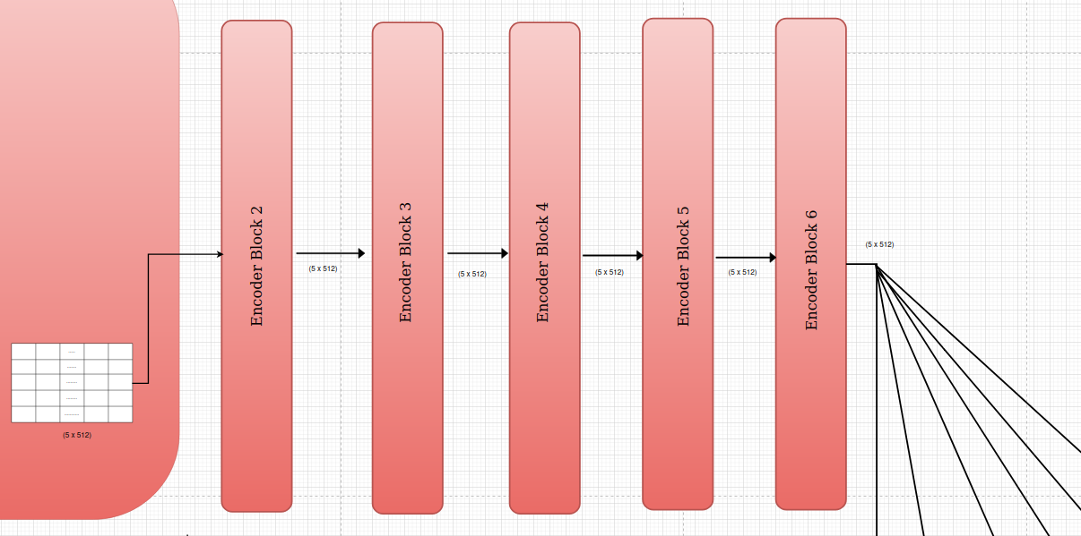
Final Output:

The final output of the encoder is a sequence of vectors, where each vector corresponds to a word in the input sequence.
These vectors capture rich contextual information about each word, incorporating its relationships and dependencies with other words in the sequence.
This final output is then used by each decoder block to generate the target sequence in tasks like machine translation.

Decoder

In the original Transformer paper, “Attention Is All You Need,” the decoder block is a crucial component responsible for processing the target sequence (e.g., the sentence being translated in machine translation) and generating the output sequence.Let’s imagine we’re translating the sentence “Nepal is a beautiful Country” from English to Nepali (“नेपाल सुन्दर देश हो”).In a machine translation example, the decoder block is responsible for:

Remembering the words it has already translated.
Taking hints from the original sentence.
Choosing the best word to translate next, making sure it fits the context and meaning of both languages.

Each components of the decoder block is discussed below:

Tokenization

As we had tokenized the input sentence before. converting it to input embedding in the encoder, we are going to tokenize the output sentence before creating its embedding to pass to the decoder layer.

Output Sentence: “नेपाल सुन्दर देश हो”

Tokenization Method: Word-based (splitting on spaces and punctuation) - for now, let’s not used punctuation of Nepali Language.

Tokens:

नेपाल
सुन्दर
देश
हो

After tokenizing, the tokens are mapped to some integer id based on the size of the vocabulary of the output language. The process is same as input ids discussed before. The mapping may look like :

नेपाल: 1256
सुन्दर :652
देश: 879
हो: 236

Input Embeddings

The integer indices are passed through an embedding layer. This layer is initialized with random values and learns to map each index to a continuous vector during training. Each index corresponds to a row in the embedding matrix, and the layer retrieves the corresponding vector for each output token.
The dimension of the input embedding vectors(embedding of the output words - Nepali words in this case) is 512 in the original transformer paper. This means that each token in the output sequence is represented by a dense vector of length 512 after passing through the embedding layer.

Positional Encodings

The positional information of each word/token in the output language is encoded/added using the same approach mentioned before encoder block above.

Masked Multi Head Attention

The masked multi-head attention block in the Transformer’s decoder is where the magic of understanding context and relationships between words truly happens.The step by step processes that happens inside masked multihead attention:

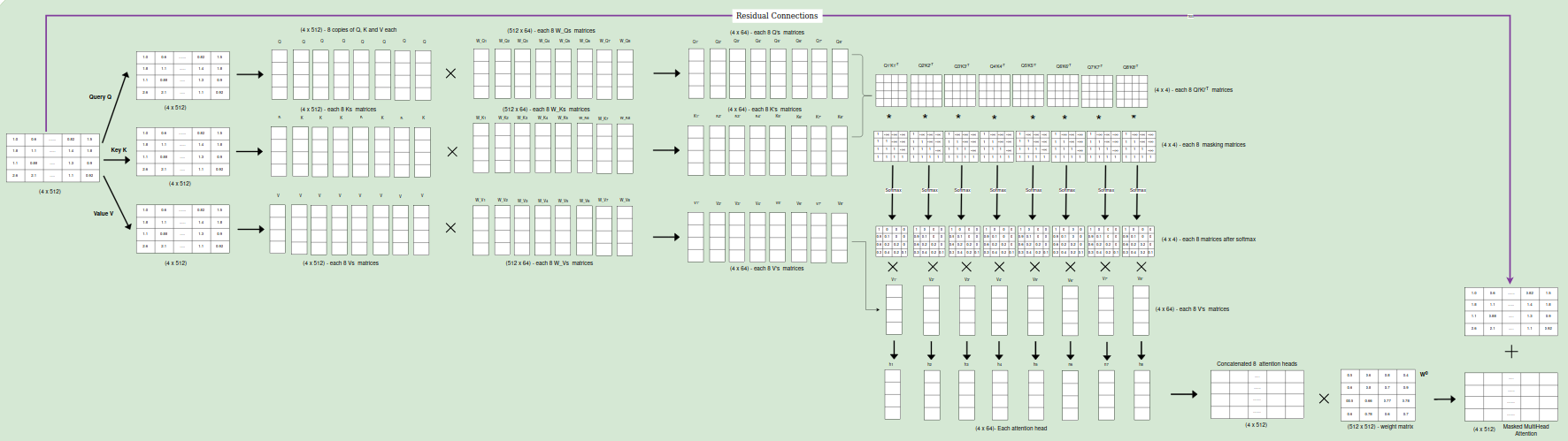
1. Creating Queries, Keys, and Values:Three matrices are created from the input embeddings: queries (Q), keys (K), and values (V).These matrices are used to calculate attention scores, which determine how much each word should attend to other words in the sequence.

2. Linear Transformation of Q,K and V matrices: When we introduce multi-head attention, the d_model(512) dimension is linearly transformed into h(8) heads, where h is another hyperparameter representing the number of attention heads.Each of the Q, K and V matrices are of size (4*512) as the number of output translated words is 4 in Nepali and the size of input embedding is 512. The queries (Q), keys (K), and values (V) are each linearly projected h times with different, learned linear projections. This means there are h sets of weight matrices: W_Qi(512,64), W_Ki(512,64), and W_Vi(512,64), each projecting Q, K, and V into a lower-dimensional space of dk(4,64), dk(4,64), and dv(4,64) dimensions, respectively. The original paper used h = 8 parallel attention layers or heads.This step is crucial for several reasons:

Dimensionality Reduction: Multiplying by the weight matrices allows us to further control and adjust the dimensionality of the queries, keys, and values for each head.This can be useful for managing computational complexity and tailoring the representation capacity of each head to the specific task.
Learning Head-Specific Representations: Each head has its own set of weight matrices (W_Q, W_K, W_V). This means each head can learn to focus on different aspects of the input sequence.For example, one head might learn to attend to words with similar syntactic roles, while another head might focus on semantic relationships or long-range dependencies.By learning distinct weight matrices, each head can extract unique and relevant information from the input sequence, enriching the overall representation learned by the model.
Linear Projections and Feature Extraction: The weight matrices act as linear projections, transforming the input embeddings and positional encodings into a space that is more suitable for attention calculations.This can be thought of as extracting relevant features from the input that are important for determining the relationships between words.These features might capture aspects such as word meaning, grammatical role, or positional information.

Splitting the dimensions allows for parallel processing across multiple heads, as each head can independently perform attention calculations with its smaller matrices.This improves computational efficiency and allows the model to learn diverse aspects of the relationships between words through different heads.However, splitting also reduces the capacity of each individual head compared to a single-head attention with the full d_model dimension.So, Choosing the number of heads (h) involves a trade-off between efficiency and capacity.More heads allow for more parallelization and diverse perspectives but also reduce the capacity of each head.The optimal number of heads depends on the specific task and dataset and is often determined through experimentation and hyperparameter tuning.

3. Masked Attention Calculation: The attention scores are calculated by taking the dot product of the query matrix with the transpose of the key matrix.A mask is applied to the attention scores to ensure that a word can only attend to words that come before it in the sequence. This prevents the model from “seeing” future words, which is important for maintaining the autoregressive property of the decoder.

4. Scaled Dot-Product Attention: The attention scores are scaled by the square root of the dimension of the key vectors to prevent them from becoming too large.The softmax function is applied to normalize the attention scores, resulting in a probability distribution.The value matrix is multiplied by the attention scores to obtain a weighted combination of the value vectors, where each word’s contribution is determined by its attention score.

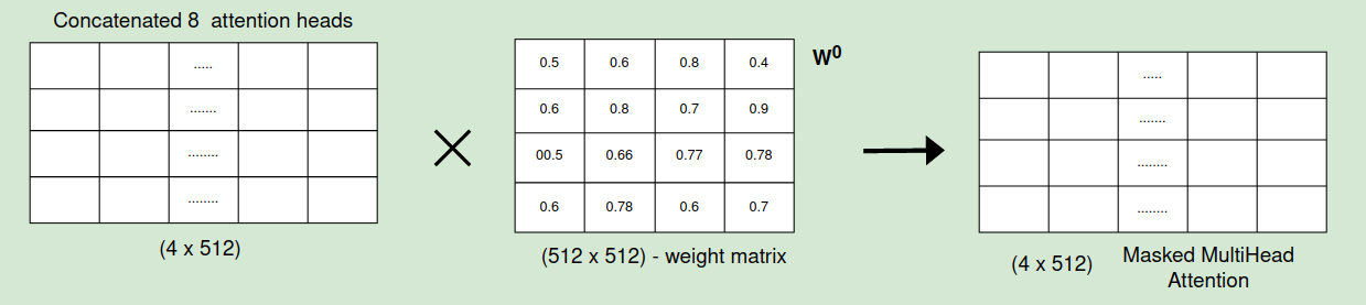
5.Multi-Head Attention:The attention mechanism is performed multiple times(8 times) in parallel, each with different sets of learned projection matrices for Q, K, and V. This allows the model to capture different aspects of the relationships between words.The outputs from each head are concatenated and linearly transformed to obtain the final output of the masked multi-head attention layer.

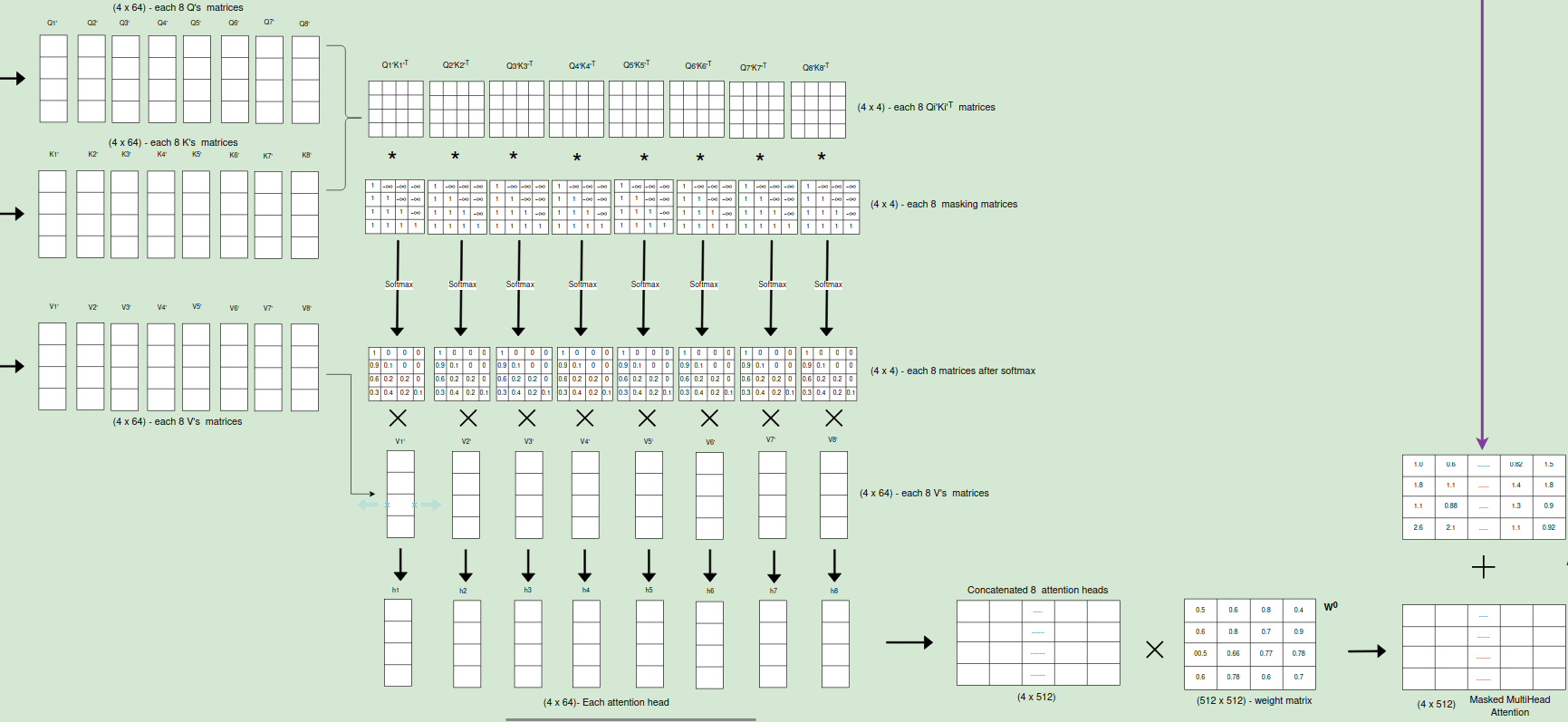
6. Output:Once each head has completed its attention calculations, the resulting vectors are concatenated, forming a single representation that incorporates information from all the different perspectives.This concatenated vector is then linearly transformed to produce the final output of the multi-head attention layer, which is passed on to the next layer in the decoder block.

Masked Multi Head Attention Concatenation

Residual Connection and Layer Normalization

Multi Head/Encoder Decoder Attention

Inputs to the Encoder Decoder Attention Block:

Queries (Q): These come from the output of the previous decoder layer. Each query represents a specific position in the output sequence for which we want to gather relevant information from the input sequence.
Memory Keys (K) and Values (V): Both come from the output of the encoder. The keys represent different positions within the input sequence, while the values contain the encoded representation of the information at those positions.

What happens inside Encoder Decoder Attention Block?

1.Linear Projections

The queries from the decoder and the keys and values from the encoder are each passed through separate linear layers. This projects them into different representation subspaces, allowing the model to capture various aspects of the information. This step results in Q’, K’, and V’ matrices.

2.Attention Calculation (per head)

Each head in the multi-head attention mechanism performs the following:

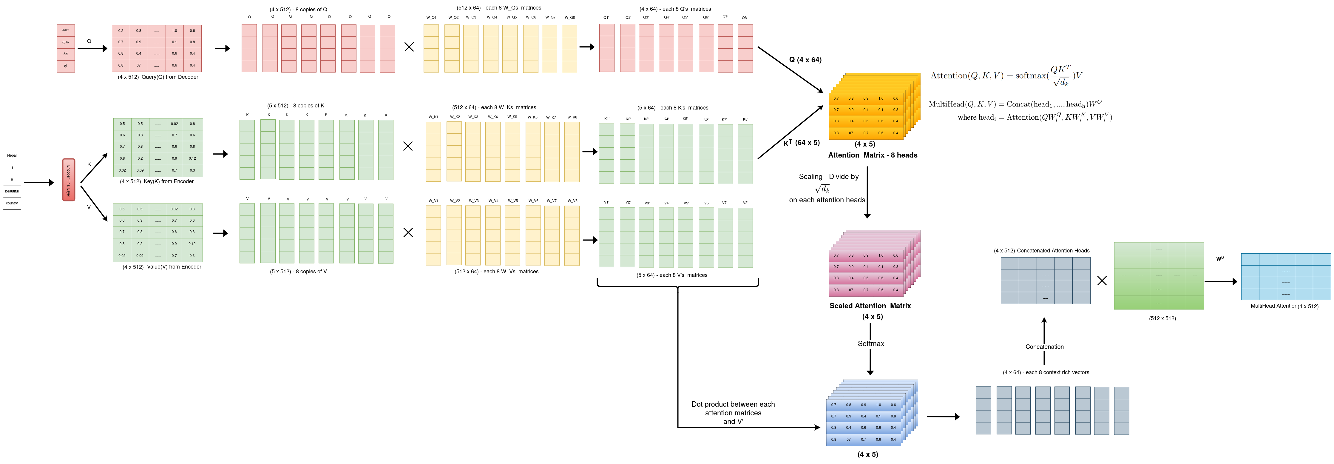
Dot Product: The dot product of the query matrix (Q’) and the key matrix (K’) is calculated. This results in a score matrix, where each element represents the similarity between a position in the output sequence (query) and a position in the input sequence (key).
Scaling: The score matrix is divided by the square root of the key dimension to prevent the values from becoming too large and ensure stable gradients during training.
Softmax: The softmax function is applied to each row of the scaled score matrix to obtain attention weights. These weights represent the importance of each position in the input sequence for the current position in the output sequence.
Weighted Sum: The attention weights are multiplied element-wise with the value matrix (V’) and the results are summed up. This produces a context vector for each position in the output sequence, containing relevant information from the input sequence based on the attention weights.

3.Concatenation

The context vectors from all the heads are concatenated to form a single matrix. This combined context vector incorporates information from different representation subspaces and attention heads, providing a richer representation of the relevant information from the input sequence.

4. Linear Transformation

A final linear layer is applied to the concatenated context matrix to produce the output of the encoder-decoder attention layer. This output is then passed on to the next layer in the decoder block.

Residual Connection and Layer Normalization

The main goal of a residual connection is to address the vanishing gradient problem, which can occur in deep neural networks. By adding the input of a layer to its output, the network can propagate gradients more effectively during training. This helps prevent gradients from becoming too small and allows for deeper architectures.Layer normalization stabilizes the distribution of activations, leading to faster convergence during training.Typically, the residual connection and layer normalization are applied immediately after the encoder-decoder attention layer, before moving on to the next layer of the decoder. This ensures that the benefits of both techniques are fully utilized in the network.

Fully Connected Neural Networks

The Feed Forward Network(FFN) within each Transformer block consists of two linear transformations with a ReLU activation function between them. The paper describes the FFN as having a hidden layer with a dimension of 2048 and an output layer with the same dimension as the input, which is 512.

Input Dimension: 512
Hidden Layer Dimension: 2048 (expansion ratio of 4)
Output Dimension: 512

Note : Expansion Ratio = Hidden Layer Dimension / Input Dimension

A higher expansion ratio allows the FFN to learn more complex and richer feature representations. It increases the model’s capacity to capture intricate relationships between input and output.The expansion followed by contraction in the FFN introduces non-linearity, which is crucial for learning non-linear patterns in the data. Increasing the expansion ratio also increases the number of parameters in the model, leading to higher computational cost and potential overfitting.The optimal expansion ratio depends on various factors like the task complexity, dataset size, and available computational resources. Common choices for the expansion ratio range from 2 to 4, but it can be adjusted based on experimentation and hyperparameter tuning.

The authors of the paper chose these dimensions based on empirical experimentation and the need for a balance between model capacity and computational efficiency. The expansion ratio of 4 allows the FFN to learn more complex features while maintaining a manageable number of parameters.

Residual Connection and Layer Normalization

The output from FFN and previous Residual and Normalized Layer is added and Normalized again. The Add & Norm layer is applied immediately after the FFN in both the encoder and decoder blocks of the Transformer. This ensures that the benefits of residual connections and layer normalization are fully utilized throughout the network.

Decoder Blocks

The paper proposes a decoder with 6 identical blocks stacked sequentially. Each block performs a similar set of operations but maintains its own set of parameters, allowing the model to learn hierarchical representations of the input sequence.

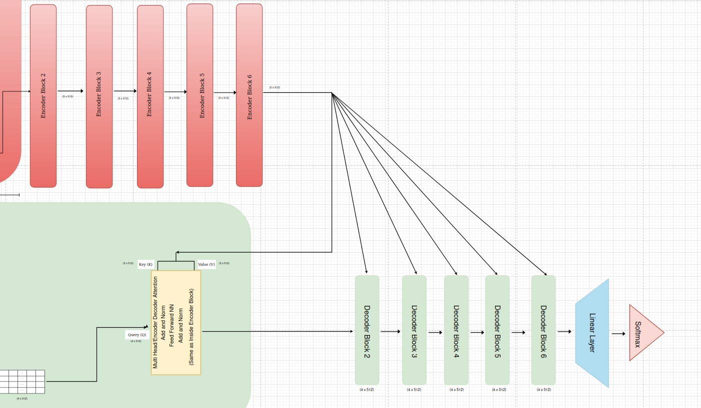
Each decoder block receives input from two primary sources:

Output of the Previous Decoder Block: The output of the preceding decoder block serves as the primary input to the current block. This allows the decoder to build upon the representations learned in previous layers, gradually refining the understanding of the input sequence and generating the output sequence step by step.
Output of the Encoder: The encoder’s final output, which represents a contextualized encoding of the source sequence, is passed to each decoder block. This information is crucial for the decoder to attend to relevant parts of the source sequence when generating the target sequence. The encoder output is specifically used within the “encoder-decoder attention” sub-layer of each decoder block.

Linear Layer

In the original Transformer paper, after the stack of 6 decoder blocks, a final Linear layer is applied to project the decoder’s output into a space with the vocabulary size dimension(45000 to 50000 in case of Nepali Language). This layer essentially transforms the decoder’s output into logits, which represent the unnormalized probabilities for each word in the vocabulary.

Functionality of the Linear Layer:

Projection: The Linear layer takes the final decoder block’s output, which is a representation of the target sequence, and projects it into a higher-dimensional space. This space has the same dimensionality as the vocabulary size, meaning each dimension corresponds to a specific word in the vocabulary.
Logits Calculation: The output of the Linear layer represents the logits for each word in the vocabulary. These logits are unnormalized probabilities, indicating the model’s preference for each word as the next token in the sequence.

Hidden and Output Layers:

The Linear layer itself does not have any hidden layers. It’s a single, fully connected layer that directly transforms the input into the output.
The output layer of the Linear layer has the same dimensionality as the vocabulary size. Each neuron in the output layer corresponds to a specific word, and its activation represents the logit (unnormalized probability) for that word.

Softmax

After the Linear layer, a softmax function is typically applied to convert the logits into probabilities. The word with the highest probability is then chosen as the next token in the generated sequence.